
A Monte Carlo portfolio simulation runs thousands of possible market futures and reports what share of them let your money last, plus the full range of outcomes above and below that line. The headline "success probability" is only an entry point.
TL;DR:
- Success probability alone is misleading; analyzing tail outcomes, especially the 10th percentile, reveals potential for early portfolio depletion.
- The choice between historical resampling, independent draws, and block-bootstrap methods significantly impacts success estimates, especially during market slumps.
- Careful calibration of return and volatility assumptions is crucial, as small shifts can greatly alter long-term simulation results.
- Rerunning simulations with lower withdrawal rates or added cash buffers can improve worst-case scenarios without sacrificing much median performance.
- Validating models against historical data and testing multiple horizons helps identify assumptions that could make plans fragile or robust.
Table of Contents
- What does a Monte Carlo portfolio simulation actually show you?
- How does the simulation actually generate those paths?
- What inputs do you need to set before running a simulation?
- How do you turn a success rate into an actual decision?
- A worked retirement example, and two quick sensitivity checks
- Where does Monte Carlo fall short, and how do you check it?
- How Alphaiq applies simulation responsibly
- Why the headline number is the least useful part of the output
- Model your own retirement numbers with Alphaiq
- Sources
What does a Monte Carlo portfolio simulation actually show you?
A Monte Carlo portfolio simulation runs your portfolio through thousands of simulated market paths, applying your withdrawals, inflation and rebalancing rules to each one, then counts how many paths still hold money at the end. This is the same technique used across finance to value and analyse investments by generating a large number of possible price paths and studying the resulting spread of outcomes.
The output isn't a single verdict. A well-built tool gives you:
- A success probability, the percentage of simulated paths that don't run out of money before the end of the horizon.
- A median path, showing the middle outcome across every simulation run.
- Percentile ranges (commonly the 10th, 25th, 75th and 90th), which reveal how bad the bad scenarios actually get.
- A histogram or scenario table showing representative paths, not just averages.
A single percentage flattens all of that into one number, which is precisely why relying on it alone is risky. Two portfolios can both show a high success rate and still carry very different tail outcomes. You only see that difference by looking past the headline figure into the distribution itself.
How does the simulation actually generate those paths?
Three broad methods dominate. Historical resampling replays real past returns, in order or shuffled, which keeps things grounded in what markets have actually done, but is limited by however many decades of data you have. A 40-year dataset gives you only so many distinct sequences to draw from.
Parametric or independent draws generate returns from assumed mean, volatility and correlation figures, usually via a normal or similar distribution. These run fast and are easy to configure, but assuming returns are independent from one period to the next understates how badly markets can cluster into extended slumps.
Block bootstrap and synthetic-path methods sample chunks of consecutive returns rather than single periods, which preserves volatility clustering and serial correlation in a way that plain independent draws cannot. That distinction matters most for retirees, because a bad run of years early in retirement does more damage than the same bad years spread evenly across three decades.
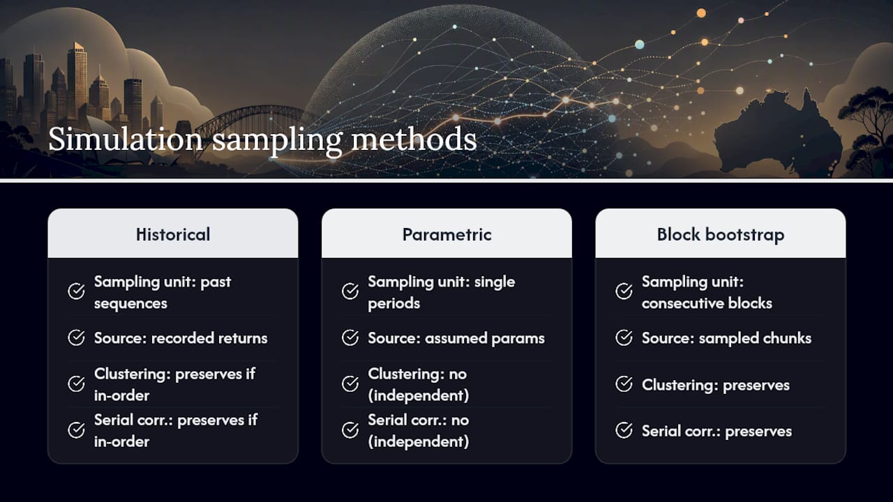
Pro Tip: If a simulator lets you toggle between independent draws and block bootstrap, run both. A material gap in success probability between the two tells you your plan is sensitive to how returns cluster, not just their average.
What inputs do you need to set before running a simulation?
Every simulation is only as good as what you feed it. Work through these in order:
- Starting balance, time horizon and withdrawal rule. Decide whether withdrawals are a fixed dollar amount, a fixed percentage, or a rule that adjusts with the portfolio's performance, and set how often withdrawals happen and how inflation gets applied.
- Asset allocation and return assumptions. Set expected return, volatility and correlation for each asset class you hold, plus your rebalancing frequency and a realistic allowance for fees and tax drag.
- Trial count and time step. Run at least a few thousand trials, and prefer monthly over annual steps for withdrawal-heavy models, since monthly steps catch sequencing effects that annual snapshots smooth over.
- Sensitivity variables. Before you trust a single result, rerun it while varying your withdrawal rate, expected return, volatility and horizon length one at a time.
Calibration matters more than people expect here. Long-horizon simulations are unusually sensitive to small shifts in assumed mean returns and time-varying volatility, which is why careful calibration of return and volatility inputs rather than naive historical averages tends to produce more defensible results. Our guide to modelling investment returns walks through setting these assumptions in more detail.
How do you turn a success rate into an actual decision?
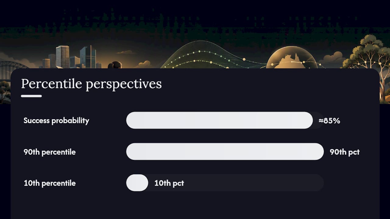
A success probability around eighty-five percent doesn't mean an equivalent chance your specific plan works. It means roughly that share of simulated paths under your chosen assumptions didn't run out of money. Change the assumptions and that number moves, sometimes sharply.
Percentiles do more work than the headline figure. The 90th percentile shows what happens if markets are kind to you; the 10th percentile shows what happens if they aren't.
Reading the tails: if your 10th percentile outcome leaves the portfolio depleted by year 20 of a 30 year retirement, that's the scenario to plan around, not the median. Per-path percentile detail matters more than the single success number precisely because it exposes that kind of gap.
Sequence-of-returns risk shows up clearly once you look at individual paths rather than the summary statistic: a portfolio that suffers a market downturn in its first five retirement years behaves very differently to one that hits the same downturn in year twenty five, even with identical average returns. Our breakdown of sequence-of-returns risk covers why timing hurts more than magnitude.
Practical responses to weak tail results include:
- Holding one to two years of withdrawals in cash to avoid selling into a downturn.
- Building in a flexible withdrawal rule that trims spending after a bad year.
- Delaying retirement by a year or two if the horizon is genuinely open.
- Shifting a modest slice of the portfolio toward defensive assets if the 10th percentile keeps disappointing across reruns.
A worked retirement example, and two quick sensitivity checks
In a typical balanced allocation, the median simulated path might leave a substantial balance at year 30, while the 10th percentile path shows the money running low well before the end. That gap between median and 10th percentile is the entire point of running the simulation in the first place.
Two adjustments are worth testing before settling on a plan:
- Drop the withdrawal rate to 3.5%. This usually lifts the success probability and narrows the gap between the median and the 10th percentile, at the cost of $5,000 a year in spending on this example balance.
- Add a defensive cash buffer. Holding two years of withdrawals in cash and trimming equity exposure slightly tends to improve the worst-case paths more than it drags on the median, because it reduces forced selling during downturns.
Neither change produces a single "correct" number. The value of running both is seeing how much the tail outcomes shift relative to the median, which tells you where your actual flexibility lies. For a broader look at trade-offs like this, see our guide on optimising a portfolio for smarter returns.
Where does Monte Carlo fall short, and how do you check it?
Every simulation carries model risk. Results depend entirely on the assumptions you fed in, and no model captures every real-world wrinkle, including sudden policy or tax changes, entitlement taper interactions, currency effects on offshore holdings, or fees that got left out of the setup.
Run these checks before trusting a result:
- Compare the Monte Carlo output against a historical rolling-window replay using the same portfolio and withdrawal rule; large disagreement between the two flags an assumption worth revisiting.
- Rerun with block-bootstrap sampling instead of independent draws and see whether the tail outcomes move.
- Test at least two horizon lengths and confirm the trial count is high enough that results don't shift noticeably between reruns.
Pro Tip: Be wary of any retail tool that shows only one success percentage with no percentile breakdown or sensitivity controls. That's a sign the model is hiding more than it's showing.
How Alphaiq applies simulation responsibly
Alphaiq builds tax-aware financial modelling and scenario simulation for Australians managing investments, superannuation, property and retirement income in one place. That matters here because a Monte Carlo result stripped of tax, franking credits and super drawdown rules tells you very little about your actual after-tax retirement income.
Alphaiq's modelling approach follows the same discipline this article has argued for: include fees and tax drag rather than ignore them, cross-check simulated outcomes against historical replay, and stress-test the tails rather than rest on a single headline percentage. If you want to run a guided, tax-aware version of this kind of modelling on your own numbers, our scenario modelling guide is a useful next step before you commit to a plan.
Why the headline number is the least useful part of the output
Most people who run their first Monte Carlo simulation fixate on the success percentage and stop there. That's backwards. The percentage is the least informative output in the whole exercise, and treating it as a forecast, rather than as one summary statistic drawn from a distribution, leads to false confidence in plans that have real weaknesses hiding in the 10th percentile.
A parametric model using independent draws will often report a higher success rate than a block-bootstrap model run on the identical portfolio, purely because it understates how simulated market volatility clusters. That gap is diagnostic information, not noise to average away.
What should come first isn't a better simulator. It's the habit of pulling apart every result: check the 10th percentile before the median, compare block-bootstrap against independent draws, and run the same scenario against historical replay to see if the models agree. Where they disagree is exactly where your plan is fragile, and that's worth more than any single number a tool hands you.
— Jonathan
Model your own retirement numbers with Alphaiq
Spreadsheets and generic online calculators can run a basic withdrawal projection, but they rarely account for franking credits, capital gains tax, debt recycling or how your superannuation drawdown interacts with your other income. Alphaiq closes that gap by combining Monte Carlo style scenario simulation with tax-aware modelling built specifically around the Australian system, so the success probability and percentile ranges you see actually reflect what lands in your pocket after tax.

If you've been running the numbers through a generic tool and wondering why the figures don't quite match your situation, that's usually why. Alphaiq's retirement projection calculator lets you set your own allocation, withdrawal rule and horizon, then stress-test the result the same way this article has walked through, tails included. Start a trial and run your own numbers before you settle on a withdrawal rate.
This article is general information, not a substitute for advice from a qualified financial advisor. Consult a qualified financial professional about your own circumstances before acting on anything here.
Sources
- Monte Carlo methods in finance — Wikipedia
- arXiv preprint (block bootstrap / synthetic path discussion)
- Monte Carlo retirement simulation: What it measures (and misses) — SuperCalc Pro