
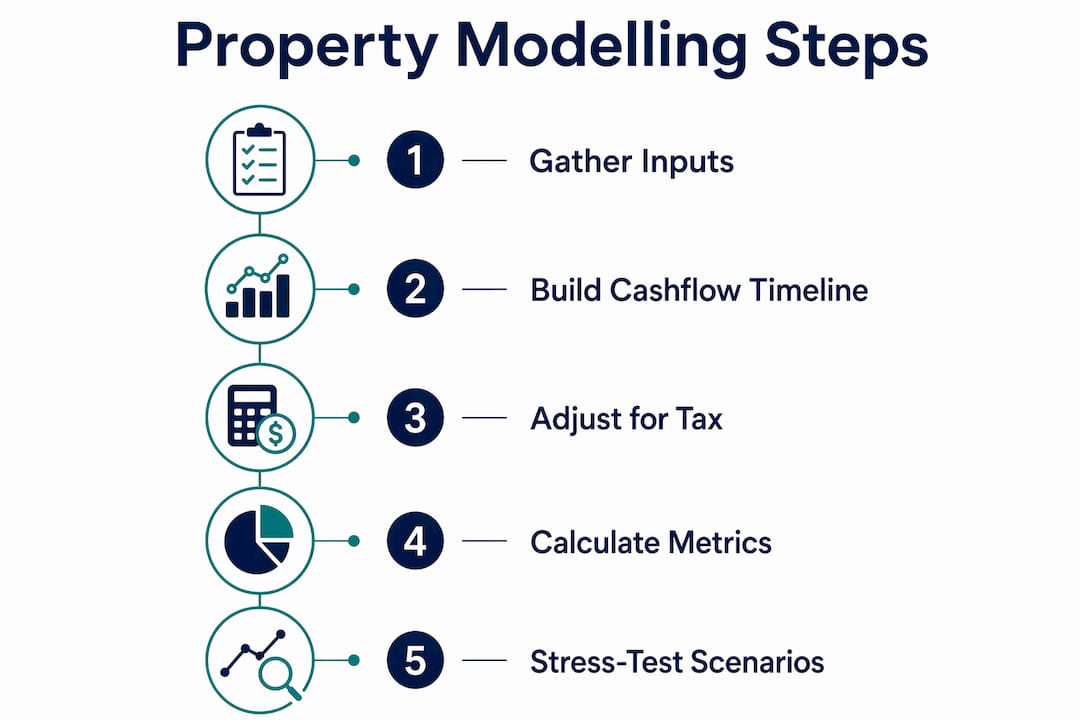
Modelling property returns in Australia comes down to six steps: collect all inputs, build a year-by-year cashflow timeline, apply Australian tax adjustments, calculate after-tax return metrics, run scenario and sensitivity tests, then interpret outputs in a portfolio context. Done properly, the model produces:
- After-tax annual cashflow (pre and post negative gearing benefit)
- Equity path from year 1 to sale
- Internal rate of return (IRR) and net present value (NPV)
- Break-even year (when cumulative after-tax cashflow turns positive)
- CGT liability at each potential sale year
This guide walks through every step using Australian tax rules, ATO references, and worked numbers. Alphaiq is the recommended platform for investors who want this modelling automated, scenario-tested, and integrated with their broader portfolio.
Table of Contents
- What inputs does your property return model need?
- How to build your year-by-year cashflow timeline
- Australian tax adjustments you must model
- Which return metrics actually matter for your decision?
- How to stress-test your model with scenarios
- Common modelling mistakes Australian investors make
- Worked 10-year example: growth property vs yield property
- What should you look for in a property modelling tool?
- Your model documentation checklist
- Key takeaways
- A practitioner's view on property modelling
- Alphaiq: tax-aware property modelling for self-directed investors
- Useful sources and further reading
What inputs does your property return model need?
A model is only as reliable as its inputs. Collect every figure below before you build a single formula.
Core numeric inputs:
- Purchase price, deposit, and stamp duty (varies by state and property value)
- Loan terms: interest rate, loan type, amortisation period
- Weekly rent and projected rent growth rate
- Vacancy allowance (typically 2–4% of gross annual rent, even in tight markets)
- Operating costs: council rates, strata levies, landlord insurance, property management fees (usually 7–10% of rent), maintenance and repairs
- Land tax (state-specific; thresholds and rates differ significantly between NSW, VIC, QLD and others)
- Depreciation: Division 43 capital works (2.5% p.a. on construction cost) and Division 40 plant and equipment
- Selling costs: agent commission (a typical percentage of sale price), legal fees, and any capital improvements to add to the cost base
- Holding period and intended sale year
Assumption inputs to document:
- Capital growth rate (conservative capital growth rate assumptions for most Australian markets)
- Expense inflation rate (2–3% p.a. on non-mortgage costs)
- Investor's marginal tax rate and Medicare levy
- Investment structure: individual, discretionary trust, or company
For market rent and growth assumptions, national data providers and local property reports are the most defensible sources. Document every assumption with its source and date so the model can be audited and updated.

How to build your year-by-year cashflow timeline
The cashflow timeline is the engine of the model. Each row is a cash item; each column is a year.
Steps to build it:
- Calculate gross annual rent (weekly rent × 52), then apply the vacancy allowance to get effective gross rent.
- Subtract operating expenses (council rates, strata, insurance, management, maintenance) to get net operating income before financing.
- Split loan repayments into interest and principal using an amortisation schedule. Interest is generally deductible; principal is not.
- Add depreciation deductions (Div 43 and Div 40) as non-cash items that reduce taxable income.
- Calculate the pre-tax net rental result (effective gross rent minus operating expenses minus interest minus depreciation).
- In the final modelled year, add sale proceeds minus selling costs and CGT liability.
Example annual cashflow table layout:
| Item | Year 1 | Year 2 | Year 5 | Year 10 |
|---|---|---|---|---|
| Net taxable rental result | ($12,280) | — | — | ($1,357) |
| Principal repayment | ($4,200) | ($4,600) | ($6,100) | ($8,400) |
| Pre-tax cashflow | ($16,480) | ($15,978) | ($14,273) | ($9,757) |
Expense inflation matters here. Modelling operating costs with an annual inflation factor rather than fixed amounts keeps long-range projections realistic; static costs overstate cashflow and produce optimistic break-even years.
Australian tax adjustments you must model
Australian tax rules change property outcomes materially. These are the adjustments every model must include.
Tax effects to model:
- Rental income is assessable at your marginal rate (up to 47% including Medicare levy)
- Deductible expenses reduce assessable income: interest, management fees, repairs, council rates, insurance, and depreciation
- Negative gearing: when deductible expenses exceed rental income, the net loss offsets other assessable income, reducing tax payable in that year
- CGT discount of 50% applies to assets held more than 12 months; only the discounted gain is taxed at your marginal rate in the sale year
- Land tax applies annually above state-specific thresholds; model it as an operating expense with the correct state rate
Worked tax calculation example (Year 1, individual investor, 37% marginal rate):
Net taxable rental result: ($12,280) loss Tax saving: $12,280 × 37% = $4,544 reduction in tax payable After-tax weekly out-of-pocket cost: ($16,480 pre-tax cashflow + $4,544 tax saving) ÷ 52 = $228 per week
The ATO's negative gearing rules mean a rental loss directly reduces your taxable income in the year it occurs. The CGT 50% discount then applies at sale for assets held over 12 months, making the timing of disposal a significant modelling variable. Always check current rates and thresholds at ato.gov.au before finalising your model.
Pro Tip: Document your investment structure before you model. An individual on a 47% marginal rate benefits more from negative gearing deductions than a company taxed at 25% or 30%, but loses access to the 50% CGT discount. A discretionary trust can distribute gains to lower-rate beneficiaries, changing the after-tax sale outcome significantly. If structure questions arise, consult a registered tax agent before committing to a purchase.
For a deeper walkthrough of negative gearing mechanics and their cashflow impact, Alphaiq's interactive calculator shows the weekly cost at different marginal rates.
Which return metrics actually matter for your decision?
Pre-tax yield is a starting point, not a decision tool. After-tax metrics are what drive real wealth outcomes.
Metrics to calculate:
- Gross rental yield: Annual rent ÷ purchase price. Simple but ignores all costs.
- Net yield: (Annual rent minus operating costs) ÷ purchase price. Net yield typically sits 1.0–1.8 percentage points below gross yield in Australian suburbs.
- After-tax net yield: Net yield adjusted for the tax saving from negative gearing.
- Cash-on-cash return: After-tax cashflow ÷ cash invested (deposit plus costs).
- IRR: The discount rate that makes NPV zero across all cashflows including sale proceeds. After-tax IRR is the most complete single metric.
- NPV: Present value of all after-tax cashflows at your chosen discount rate.
- Equity accumulation: Property value minus outstanding loan at each year.
- Break-even year: When cumulative after-tax cashflow (including tax savings) turns positive.
A property can show positive pre-tax cashflow yet deliver a poor after-tax IRR once non-deductible principal repayments and a modest growth rate are included. Running multiple return metrics together reveals these conflicts before you commit capital.
Over a 10-year hold, capital growth typically drives the largest share of total return, with rental income and tax benefits contributing meaningful but smaller portions. That sensitivity to growth assumptions is exactly why scenario testing matters.
How to stress-test your model with scenarios
A single base-case projection is not a plan. Scenario testing shows which assumptions drive outcomes and where your model breaks.
Scenario types to run:
- Base case: Your central assumptions (e.g., 4.5% capital growth, 3% rent growth, current interest rate)
- Optimistic: 6% growth, 4% rent growth, stable rates
- Downside: 2% growth, 1% rent growth, 1% vacancy increase
- Interest shock: Base case plus a 1.5–2 percentage point rate rise
- Vacancy spike: Base case with vacancy rising to 8–10% for two years
- Low growth: 2–3% capital growth sustained for the full hold period
For one-variable sensitivity, run a tornado analysis: hold all other inputs constant and shift each variable by a defined amount. Growth rate and interest rate typically dominate outcomes; vacancy and management costs have a smaller but compounding effect.
Pro Tip: Run scenarios at the portfolio level, not just per property. Adding a second property changes your total rental income, which can push you into a higher marginal tax bracket or reduce the benefit of negative gearing on the first property. Alphaiq's scenario engine computes tax holistically across all holdings, so bracket interactions are visible before you act.
Common modelling mistakes Australian investors make
Most errors are predictable and fixable before they distort a decision.
- Static operating costs: Fixing council rates, insurance, and strata at Year 1 amounts overstates cashflow by Year 5 and beyond. Apply a 2–3% annual inflation factor.
- No vacancy allowance: Even a 98% occupancy market has turnover gaps. A 3% vacancy allowance on gross rent is a minimum; always include it regardless of local conditions.
- Ignoring lender shading: Lenders typically assess only 80% of gross rent for serviceability purposes. Model this when testing borrowing capacity under rate shocks.
- Treating the full repayment as a cost: Only the interest component is deductible. Principal repayment is a balance sheet movement, not a tax deduction.
- Forgetting land tax: State land tax thresholds and rates vary widely. NSW, VIC, and QLD each apply different rules; omitting land tax understates annual holding costs.
- Mis-treating depreciation: Post-9 May 2017 rules restrict Div 40 deductions on second-hand plant for residential property. New builds retain full Div 40 access.
A red flag in any model: steady positive cashflow projections combined with declining equity or an unrealistic 7%+ growth assumption held flat for 10 years.
Worked 10-year example: growth property vs yield property
Two hypothetical properties, same $650,000 purchase price, same 80% LVR, same investor on a 37% marginal rate.
| Metric | Growth property (4% yield, 6% growth) | Yield property (6% yield, 3% growth) |
|---|---|---|
| Year 1 net taxable result | ($14,200) loss | ($3,800) loss |
| Year 1 tax saving | $5,254 | $1,406 |
| Year 1 after-tax weekly cost | $171 | $45 |
| Property value at Year 10 | $1,163,000 | $874,000 |
| Equity at Year 10 | $703,000 | $414,000 |
| Cumulative after-tax cashflow | ($68,000) | ($14,000) |
| CGT payable at Year 10 sale | $95,000 (approx.) | $42,000 (approx.) |
| After-tax total wealth gain | $540,000 | $358,000 |
| After-tax IRR | 9.1% | 6.8% |
The growth property costs more each week and produces a larger CGT bill, but delivers $182,000 more in after-tax wealth over 10 years for this investor. The yield property suits an investor who needs cashflow neutrality now, perhaps because their income is already near the top marginal bracket or their serviceability is constrained.
The CGT timing decision is often worth more than the property selection itself. Selling in a year when your other income is lower, or after a partial retirement, can reduce the effective CGT rate by 5–10 percentage points on the discounted gain. Model multiple sale years, not just Year 10.
- The growth property's negative gearing benefit is largest in the early years, then narrows as rent rises and interest falls.
- The yield property reaches cashflow neutrality around Year 4; the growth property around Year 7.
- Both benefit from the 50% CGT discount at sale, held well beyond 12 months.
What should you look for in a property modelling tool?
Essential feature checklist:
- Multi-year cashflow projection (10+ years)
- Amortisation schedule separating interest and principal
- Tax module covering negative gearing, marginal rates, Medicare levy, and CGT discount
- Depreciation schedules (Div 43 and Div 40, with post-2017 restrictions)
- Scenario and sensitivity engine
- Portfolio aggregation with holistic tax calculation across all properties
- Exportable reports for accountants and brokers
A spreadsheet gives you full control and auditability but requires you to build and maintain the tax logic yourself. Online calculators are fast but rarely handle portfolio-level tax interactions. A dedicated platform like Alphaiq combines the depth of a spreadsheet with automated tax modelling, scenario simulation, and portfolio aggregation, without requiring you to rebuild the engine each time assumptions change.
Your model documentation checklist
A model without documentation is a model you cannot trust six months later.
- Assumption table: Every input with its source, date, and rationale (e.g., "4.5% growth rate — CoreLogic 10-year suburb median, accessed March 2026")
- Tax rules applied: ATO references for negative gearing treatment, CGT discount eligibility, and depreciation rules used
- Lender shading assumption: State which shading rate was used (e.g., 80% of gross rent) and why
- Depreciation schedules: Quantity surveyor report reference or estimate basis
- Scenario definitions: Name, inputs changed, and rationale for each scenario run
- Version and date stamp: Every saved version labelled with the date and what changed
When sharing a model with an accountant or mortgage broker, the assumption table and tax rules section are the two items they will scrutinise first.
Key takeaways
Modelling property returns after tax, with documented assumptions and scenario testing, is the single most reliable way to compare Australian investment properties on equal footing.
| Point | Details |
|---|---|
| Model after-tax, not pre-tax | After-tax IRR and net yield account for negative gearing and CGT discount, which materially change the decision for investors on higher marginal rates. |
| Include vacancy and expense inflation | A 3% vacancy allowance and 2–3% annual cost inflation keep long-range projections realistic and prevent overstated break-even years. |
| Stress-test interest and growth | An interest shock of 1.5–2 percentage points and a low-growth scenario of 2–3% p.a. reveal whether the investment survives adverse conditions. |
| Document every assumption | Record the source, date, and rationale for each input so the model is auditable and comparable across properties and time. |
| Use Alphaiq for portfolio modelling | Alphaiq automates tax-aware cashflow, scenario simulation, and portfolio aggregation so you can model multiple properties with holistic tax treatment in one place. |
A practitioner's view on property modelling
Most investors I see come to modelling too late, after they have already committed to a purchase. The model then becomes a justification exercise rather than a decision tool. The investors who get the most from this process run their base case and their downside scenario before they make an offer, not after. What consistently surprises them is how much the tax structure and the sale year timing matter relative to the property selection itself. A growth suburb with a well-timed disposal can outperform a higher-yield property by a margin that dwarfs the difference in weekly cashflow. Alphaiq was built precisely for this kind of analysis: tax-aware, scenario-driven, and integrated across your whole portfolio so you can see the full picture before you act. If you want to go deeper on tax-aware investing strategies and how they interact with property returns, the Alphaiq blog has detailed guides and worked examples.
Alphaiq: tax-aware property modelling for self-directed investors
Serious property modelling requires more than a yield calculator. Alphaiq gives Australian self-directed investors a complete tax-aware modelling platform: multi-year cashflow projections, an amortisation engine that separates interest from principal, a tax module covering negative gearing and the CGT discount, Division 43 and 40 depreciation schedules, a scenario simulator, and portfolio aggregation with holistic tax treatment across all your holdings.

The difference from a generic spreadsheet is that Alphaiq computes tax at the portfolio level, so bracket interactions and Medicare levy impacts are accurate when you add a second or third property. Reports are exportable for your accountant or broker. If you want to model your next purchase, run a downside scenario, or see how your property portfolio interacts with your super projections, start with Alphaiq and run your first model today. You can also use the superannuation calculator to integrate property wealth with your retirement income projections.
Useful sources and further reading
- ATO: Property and capital gains tax — primary reference for CGT discount eligibility, cost base rules, and record-keeping requirements
- State revenue offices (Revenue NSW, State Revenue Office Victoria, Queensland Revenue Office) — for current land tax thresholds and rates by state
- Rental yield benchmarks and gross-to-net gap analysis — for calibrating yield assumptions by suburb
- Lender shading and serviceability conventions — for stress-testing borrowing capacity
- Alphaiq guides: tax tips for property investors, negative gearing explained, and top tax strategies for Australian investors
Tax rates, land tax thresholds, and depreciation rules change. Check ato.gov.au and your relevant state revenue office before finalising any model, and update your assumption table whenever a legislative change affects your inputs.
This article provides general information only and does not constitute financial, tax, or legal advice. Confirm current rates and rules with the ATO, your state revenue office, or a qualified tax agent for your specific situation.